
Get Started
Tensor
Pytorch is similar with Numpy, but tensor can be accelerated on GPU.
import torch
import numpy as np

numpy_tensor = np.random.randn(2,3)
# Numpy ndarry -> PyTorch Tensor
pytorch_tensor1 = np.Tensor(numpy_tensor)
pytorch_tensor2 = np.from_numpy(numpy_tensor)

# get the shape of the tensor
pytorch_tensor1.shape
pytorch_tensor1.size()

# get the datatype of the tensor
pytorch_tensor1.type()

# get the dimension of the tensor
pytorch_tensor1.dim()

# get the number of all elements in the tensor
pytorch_tensor1.numel()

# create a matrix, which elements are 1 and size is (2,3)
x = torch.ones(2,3)

# create a matrix with random value
x = torch.randn(4,3)

# get the largest value in each row
max_value, max_idx = torch.max(x, dim=1)

# get sum for each row
sum_x = torch.sum(x,dim=1)
Variable
Variable is encapsulation of tensor. There’re three attributes of Variable:.data .grad .grad_fn.
from torch.autograd import Variable
x_tensor = torch.randn(10,5)
y_tensor = torch.randn(10,5)

# tensor -> Variable
x = Variable(x_tensor, requires_grad = True) # require computing gradient
y = Variable(y_tensor, requires_grad = True)

z = torch.sum(x+y)
print(z.data)
print(z.grad_fn)

z.backward()
print(x.grad)
print(y.grad)
Automatically Derivation
import torch
from torch.autograd import Variable

x = Variable(torch.Tensor([2]),requires_grad=True)
y = x + 2
z = y**2 +3
z.backward()
print(x.grad)

x = Variable(torch.randn(10,20), requires_grad=True)
y = Variable(torch.randn(10,5), requires_grad=True)
w = Variable(torch.randn(20,5), requires_grad=True)

# torch.matmul is matrix multiplication
# torch.mean is to get the avgerage value
out = torch.mean(y - torch.matmul(x,w))
out.backward()
Linear Modle & Gradient descent
To the opposite direction of the gradient, we can get the minimum point by updating the value of w and b, till the best w and b with the minimum loss.
Learning rate means “stride”. A large learning rate may causes convergence hardly. A small learning rate may causes waste of time.
import torch
import numpy as np
from torch.autograd import Variable
import matplotlib.pyplot as plt

x_train = np.array([[3.3], [4.4], [5.5], [6.71], [6.93], [4.168],
                    [9.779], [6.182], [7.59], [2.167], [7.042],
                    [10.791], [5.313], [7.997], [3.1]], dtype=np.float32)

y_train = np.array([[1.7], [2.76], [2.09], [3.19], [1.694], [1.573],
                    [3.366], [2.596], [2.53], [1.221], [2.827],
                    [3.465], [1.65], [2.904], [1.3]], dtype=np.float32)

plt.plot(x_train, y_train,'bo')

x_train = torch.Tensor(x_train)
y_train = torch.Tensor(y_train)

w = Variable(torch.randn(1), requires_grad=True)
b = Variable(torch.randn(1), requires_grad=True)

x_train = Variable(x_train)
y_train = Variable(y_train)

def linear_modedl(x):
    return x * w + b

y_ = linear_model(x_train)
plt.plot(x_train.data.numpy(), y_train.data.numpy(), 'bo', label='real')
plt.plot(x_train.data.numpy(), y_.data.numpy(), 'ro', label='estimated')
plt.legend()
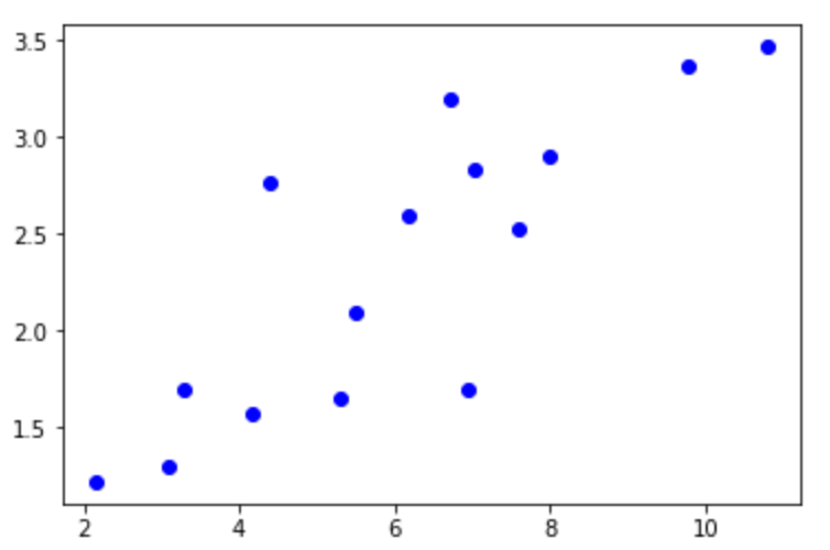
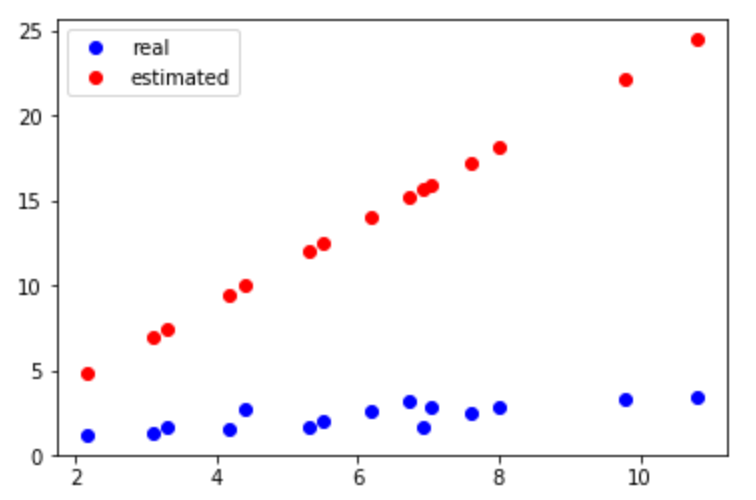
The left img shows the original data. The right img shows the result that only updates w and b by one time.
def get_loss(y_, y_train):
    return torch.mean((y_ - y_train) ** 2)

loss = get_loss(y_, y_train)
loss.backward()
w.data = w.data - 1e-2 * w.grad.data
b.data = b.data - 1e-2 * b.grad.data

for i in range(10):
    y_ = linear_model(x_train)
    loss = get_loss(y_,y_train)

    w.grad.zero_()
    b.grad.zero_()
    loss.backward()
    w.data = w.data - 1e-2 * w.grad.data
    b.data = b.data - 1e-2 * b.grad.data
    print('epoch: {}, loss: {}'.format(i, loss.data[0]))

y_ = linear_model(x_train)
plt.plot(x_train.data.numpy(), y_train.data.numpy(), 'bo', label='real')
plt.plot(x_train.data.numpy(), y_.data.numpy(), 'ro', label='estimated')
plt.legend()
plt.show()
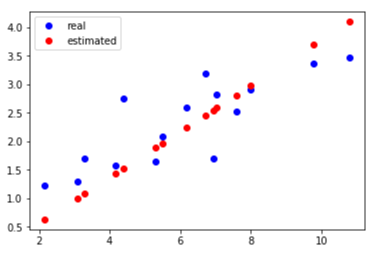
We can see the final result completes linear regression.
Below is something about plt()
Various line types, plot symbols and colors may be obtained with
    plot(X,Y,S) where S is a character string made from one element
    from any or all the following 3 columns:

             b     blue          .     point              -     solid
             g     green         o     circle             :     dotted
             r     red           x     x-mark             -.    dashdot
             c     cyan          +     plus               --    dashed
             m     magenta       *     star             (none)  no line
             y     yellow        s     square
             k     black         d     diamond
             w     white         v     triangle (down)
                                 ^     triangle (up)
                                 <     triangle (left)
                                 >     triangle (right)
                                 p     pentagram
                                 h     hexagram
Initial Parameters
import numpy as np
import torch
from torch import nn


class sim_net(nn.Module):
    def __init__(self):
        super(sim_net, self).__init__()
        self.l1 = nn.Sequential(
            nn.Linear(30, 40),
            nn.ReLU()
        )

        self.l1[0].weight.data = torch.randn(40, 30) # initial for one layer

        self.l2 = nn.Sequential(
            nn.Linear(40, 50),
            nn.ReLU()
        )

        self.l3 = nn.Sequential(
            nn.Linear(50, 10),
            nn.ReLU()
        )

    def forward(self, x):
        x = self.l1(x)
        x =self.l2(x)
        x = self.l3(x)
        return x

for i in net2.children():
    print(i)

for i i in net2.modules():
    print(i)

for layer in net2.modules():
    if isinstance(layer, nn.Linear):
        param_shape = layer.weight.shape
        layer.weight.data = torch.from_numpy(np.random.normal(0, 0.5, size=param_shape))
torch.nn.init
from torch.nn import init
print(net2[0].weight)
init.wavier_uniform(net2[0].weight)
Batch/Dataloader
Dataloader is the tool to package data, firstly we should convert data from numpy array or other format to Tensor, and then put it in the Dataloader. It can help us iterate data efficiently.
MNIST
Image.shape = [1,28,28]
import os
import torch
import torch.nn as nn
from torch.autograd import Variable
import torch.utils.data as Data
import torchvision
import matplotlib.pyplot as plt
import numpy as np

torch.manual_seed(1)

EPOCH = 5
BATCH_SIZE = 50
LR = 0.001
DOWNLOAD_MNIST = False

train_data = torchvision.datasets.MNIST(
    root = './mnist',
    train=True,
    transform = torchvision.transforms.ToTensor(),
    download = DOWNLOAD_MNIST,
)

test_data = torchvision.datasets.MNIST(root = './mnist', train=False)

train_loader = Data.DataLoader(dataset = train_data, batch_size=BATCH_SIZE, shuffle=True)

test_x = Variable(torch.unsqueeze(test_data.test_data, dim=1), volatile=True).type(torch.FloatTensor)[:2000]/255.   # shape from (2000, 28, 28) to (2000, 1, 28, 28), value in range(0,1)
test_y = test_data.test_labels[:2000]


class CNN(nn.Module):
    def __init__(self):
        super(CNN, self).__init__()
        self.conv1 = nn.Sequential(
            nn.Conv2d(
                in_channels=1,
                out_channels=16,
                kernel_size=5,
                stride=1,
                padding=2,
            ),
            nn.ReLU(),
            nn.MaxPool2d(2),
        )
        self.conv2 = nn.Sequential(
            nn.Conv2d(16,32,5,1,2),
            nn.ReLU(),
            nn.MaxPool2d(2),
        )
        self.out = nn.Linear(32*7*7, 10)

    def forward(self,x):
        x = self.conv1(x)
        x = self.conv2(x)
        x = x.view(x.size(0),-1)
        output = self.out(x)
        return output


cnn = CNN()

optimizer = torch.optim.Adam(cnn.parameters(),lr = LR)
loss_func = nn.CrossEntropyLoss()

losses = []
acces = []

for epoch in range(EPOCH):
    train_loss = 0
    train_acc = 0
    for count,(x,y) in enumerate(train_loader):

        b_x = Variable(x)

        b_y = Variable(y)

        output = cnn(b_x)

        loss = loss_func(output, b_y)
        optimizer.zero_grad()
        loss.backward()
        optimizer.step()

        train_loss += loss.data[0]

        pred = torch.max(output,1)[1]
        num_correct = (pred == b_y).sum().data[0]
        acc = num_correct/b_x.shape[0]
        train_acc += acc

    losses.append(train_loss/len(train_loader))
    acces.append(train_acc/len(train_loader))
    print('EPOCH:',epoch,',train loss:',train_loss/len(train_loader),',train acc:',train_acc/len(train_loader))

plt.title('train acc')
plt.plot(np.arange(len(acces)), acces)
plt.show()
CIFAR10
import numpy as np
import torch
from torch import nn
from torch.autograd import Variable
from torchvision.datasets import CIFAR10

torch.manual_seed(1)

def data_tf(x):
    x = np.array(x, dtype='float32') / 255
    x = (x - 0.5) / 0.5
    x = x.transpose((2, 0, 1))
    x = torch.from_numpy(x)
    return x


train_set = CIFAR10('./data', train=True, transform=data_tf)
train_data = torch.utils.data.DataLoader(train_set, batch_size=64, shuffle=True)
test_set = CIFAR10('./data', train=False, transform=data_tf)
test_data = torch.utils.data.DataLoader(test_set, batch_size=128, shuffle=False)


class VGG(nn.Module):
    def __init__(self):
        super(VGG,self).__init__()
        self.conv1 = nn.Sequential(
            nn.Conv2d(
                in_channels=3,
                out_channels=64,
                kernel_size=3,
                stride=1,
                padding=1,
            ),
            nn.ReLU(),
            nn.MaxPool2d(kernel_size=2)
        )
        self.conv2 = nn.Sequential(
            nn.Conv2d(64, 128, 3, 1, 1),
            nn.ReLU(),
            nn.MaxPool2d(2)
        )
        self.conv3 = nn.Sequential(
            nn.Conv2d(128, 256, 3, 1, 1),
            nn.ReLU(),
            nn.Conv2d(256, 256, 3, 1, 1),
            nn.ReLU(),
            nn.MaxPool2d(2)
        )
        self.conv4 = nn.Sequential(
            nn.Conv2d(256, 512, 3, 1, 1),
            nn.ReLU(),
            nn.Conv2d(512, 512, 3, 1, 1),
            nn.ReLU(),
            nn.MaxPool2d(2)
        )
        self.conv5 = nn.Sequential(
            nn.Conv2d(512, 512, 3, 1, 1),
            nn.ReLU(),
            nn.Conv2d(512, 512, 3, 1, 1),
            nn.ReLU(),
            nn.MaxPool2d(2)
        )
        self.fc = nn.Sequential(
            nn.Linear(512, 100),
            nn.ReLU(),
            nn.Linear(100, 10)
        )

    def forward(self, x):
            x = self.conv1(x)
            x = self.conv2(x)
            x = self.conv3(x)
            x = self.conv4(x)
            x = self.conv5(x)
            x = x.view(x.shape[0], -1)
            x = self.fc(x)
            return x


net = VGG()


optimizer = torch.optim.SGD(net.parameters(), lr=1e-1)
criterion = nn.CrossEntropyLoss()


def train(net, train_data, valid_data, num_epochs, optimizer, criterion):
    for epoch in range(num_epochs):
        train_loss = 0
        train_acc = 0

        for im, label in train_data:

            im = Variable(im)

            label = Variable(label)

            output = net(im)
            loss = criterion(output, label)

            optimizer.zero_grad()
            loss.backward()
            optimizer.step()

            train_loss += loss.data[0]

            pred = torch.max(output,1)[1]
            num_correct = (pred == label).sum().data[0]
            acc = num_correct/im.shape[0]
            train_acc += acc

            # train_acc += get_acc(output, label)
    print('EPOCH:',epoch,',train loss:',train_loss/len(train_data),',train acc',train_acc/len(train_data))


train(net,train_data,test_data,10,optimizer,criterion)